A Text Analysis of Women Clothing Reviews

In this study, I present a practice of natural language processing using a Women Clothing Reviews dataset downloaded from Kaggle.

Step1, load the data and take a look.

df = pd.read_csv('women_clothing_review.csv')
df.head()

Step2, preprocess and visualize the data.

Check missing values:

df.isnull().sum()
Unnamed: 0                    0
Clothing ID                   0
Age                           0
Title                      3810
Review Text                 845
Rating                        0
Recommended IND               0
Positive Feedback Count       0
Division Name                14
Department Name              14
Class Name                   14
dtype: int64

Since Title has 3810 missing values, I decided to combine Title and Review Text together as a new variable named text.

df = df.fillna('')df['text'] = df['Title'].str.cat(df['Review Text'], sep=' ')

# Check missing value for the new feature: 
df['text'].isnull().shape
(23486,)
## keep the original columns of Title and Reviews in case need them.
df.columns
Index(['Unnamed: 0', 'Clothing ID', 'Age', 'Title', 'Review Text', 'Rating','Recommended IND', 'Positive Feedback Count', 'Division Name','Department Name', 'Class Name', 'text'],dtype='object')

Check the distribution of the target variable Recommended IND. 82% of the values are 1, positive.

df['Recommended IND'].value_counts(normalize=True).round(3)
1    0.822
0    0.178
Name: Recommended IND, dtype: float64

Visualize the data by features.

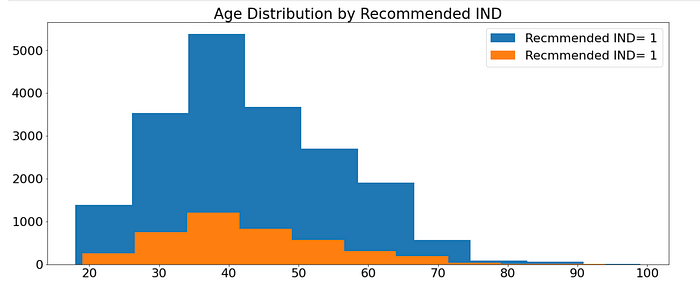
# check distribution of Age by Recommended IND
fig, ax = plt.subplots(figsize=(20, 8))
plt.hist(df[df['Recommended IND']==1]['Age'], label='Recmmended IND= 1')
plt.hist(df[df['Recommended IND']==0]['Age'], label='Recmmended IND= 1')
plt.title('Age Distribution by Recommended IND')
plt.legend()
plt.show()

# check distribution of Positive Feedback Count by Recommended IND
fig, ax = plt.subplots(figsize=(12, 8))
plt.hist(df[df['Recommended IND']==1]['Positive Feedback Count'], label='Recmmended IND= 1')
plt.hist(df[df['Recommended IND']==0]['Positive Feedback Count'], label='Recmmended IND= 1')
plt.title('Distribution of Positive Feedback Count by Recommended IND')
plt.legend()
plt.show()

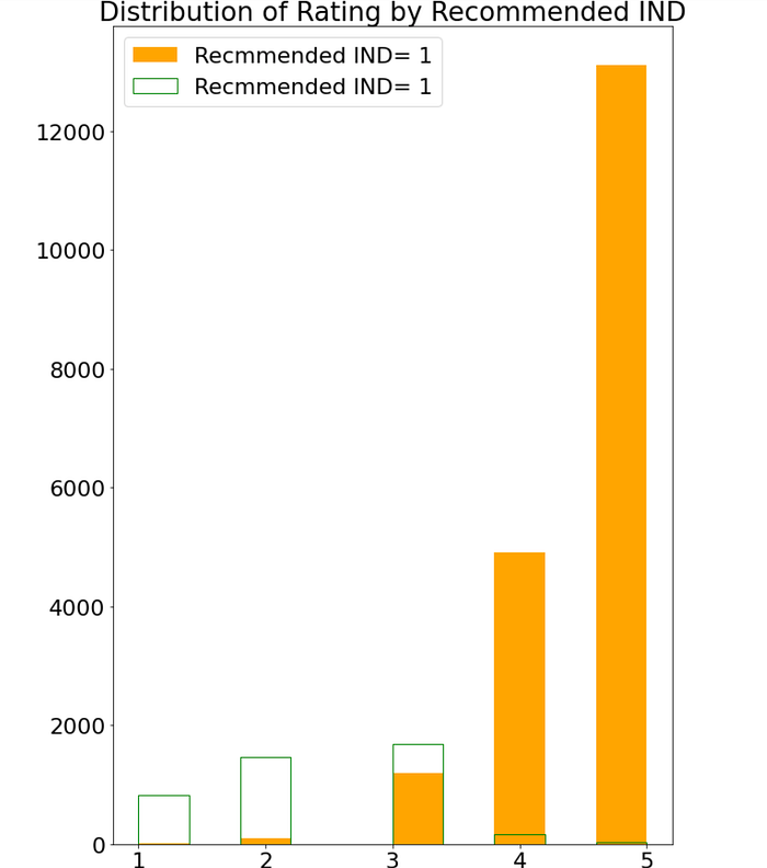
# check distribution of Rating by Recommended IND
fig, ax = plt.subplots(figsize=(10, 15))
plt.hist(df[df['Recommended IND']==1]['Rating'], label='Recmmended IND= 1', color = 'orange')
plt.hist(df[df['Recommended IND']==0]['Rating'], label='Recmmended IND= 1', histtype='step', color = 'green')
plt.title('Distribution of Rating by Recommended IND')
plt.legend()
plt.show()

# check distribution of Division by Recommended IND
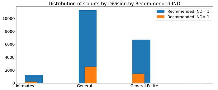
fig, ax = plt.subplots(figsize=(20, 8))
plt.hist(df[df['Recommended IND']==1]['Division Name'], label='Recmmended IND= 1')
plt.hist(df[df['Recommended IND']==0]['Division Name'], label='Recmmended IND= 1')
plt.legend()
plt.show()

# check distribution of count by Department and Recommended IND
fig, ax = plt.subplots(figsize=(20, 8))
plt.hist(df[df['Recommended IND']==1]['Department Name'], label='Recmmended IND= 1')
plt.hist(df[df['Recommended IND']==0]['Department Name'], label='Recmmended IND= 1')
plt.legend()
plt.show()

# check distribution of count by Class and Recommended IND
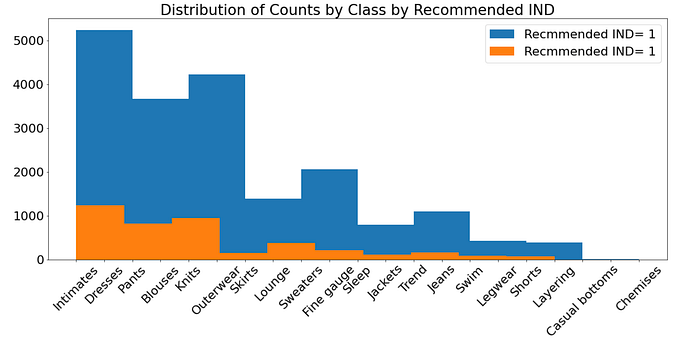
fig, ax = plt.subplots(figsize=(20, 8))
plt.hist(df[df['Recommended IND']==1]['Class Name'], label='Recmmended IND= 1')
plt.hist(df[df['Recommended IND']==0]['Class Name'], label='Recmmended IND= 1')
plt.legend()
plt.show()

Step3, preprocess text data.

In the NLP, the first step is to clean the data so that the data is usable for vectorization. The data clean for text data includes:

1. make all lower case

2. Remove punctuation, numbers, symbols, etc

3. Remove stop words, perhaps develop custom stop words list

4. Stemming/Lemmatization

Clean data by lowering text, removing punctuation, non sensical text, and space.

def clean_text_round1(text):
    '''Make text lowercase, remove text in square brackets, remove punctuation and remove words containing numbers.'''
    text = text.lower()
    text = re.sub('\[.*?\]', '', text)
    text = re.sub('[%s]' % re.escape(string.punctuation), '', text)
    text = re.sub('\w*\d\w*', '', text)
    return text
round1 = lambda x: clean_text_round1(x)
data_clean = pd.DataFrame(data_clean.text.apply(round2))
def clean_text_round2(text):
    '''Get rid of some additional punctuation and non-sensical text that was missed the first time around.'''
    text = re.sub('[‘’“”…]', '', text)
    text = re.sub('\n', '', text)
    return text
round2 = lambda x: clean_text_round2(x)
data_clean = pd.DataFrame(data_clean.text.apply(round2))

Since sklearn.feature_extraction.text.TfidfVectorizer and CountVectorizer include stop words and tokenizer_porter (used for stemming, I will use these directly)

Step4 Transforming Words into Feature Vectors

from sklearn.feature_extraction.text import CountVectorizer
from sklearn.feature_extraction.text import TfidfVectorizer
cv = CountVectorizer(stop_words='english')
# tokenize and build vocab
cv.fit(data_clean.text)
# encode document
data_cv = cv.transform(data_clean.text)
data_dtm = pd.DataFrame(data_cv.toarray(), columns=cv.get_feature_names())
data_dtm.index = data_clean.index
print(data_cv.shape)
print(type(data_cv))
(23486, 19371)
<class 'scipy.sparse.csr.csr_matrix'>

Write a function to visualize the top 20 unigram or 3-grams in the text.

# define a function to find the top20 n-grams:
def top_n_ngram(corpus,n = None,ngram = 1):
    vec = CountVectorizer(stop_words = 'english',ngram_range=(ngram,ngram)).fit(corpus)
    words_bag = vec.transform(corpus) #Have the count of  all the words for each review
    sum_words = words_bag.sum(axis =0) #Calculates the count of all the word in the whole review
    words_freq = [(word,sum_words[0,idx]) for word,idx in vec.vocabulary_.items()]
    words_freq = sorted(words_freq,key = lambda x:x[1],reverse = True)
    return words_freq[:n]

Visualize the top20 unigrams:

# visualize the top 20 unigrams:
pop_words = top_n_ngram(data_clean['text'], 20,1)
df = pd.DataFrame(pop_words, columns = ['ReviewText' , 'count'])
plt.figure(figsize =(20,6))
df.groupby('ReviewText').sum()['count'].sort_values(ascending=False).plot(
kind='bar', title='Top 20 unigrams in review after removing stop words')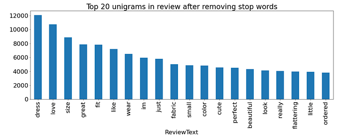

Visualize the top 20 2- grams:

Visualize the top 20 3-grams:

Visualize the top 20 5-grams:

As we can see that, the size fit is the most frequently used words in the reviews.

Now let’s build a logistic regression model that uses the vectorization of the text to predict the Recommended IND.

tfidf = TfidfVectorizer(use_idf=True)
token = tfidf.fit_transform(df['text'])
first_vector_tfidfvectorizer=token[0]
tfidf_df = pd.DataFrame(first_vector_tfidfvectorizer.T.todense(), index=tfidf.get_feature_names(), columns=["tfidf"]) 
tfidf_df = tfidf_df.sort_values(by=["tfidf"],ascending=False)[:10]
from sklearn.linear_model import LogisticRegression
from sklearn.metrics import accuracy_score, confusion_matrix, roc_auc_score
X_train = token[:20000]
X_test = token[20000:]
y_train = df['Recommended IND'][:20000].values
y_test = df['Recommended IND'][20000:].values
lr = LogisticRegression(random_state=1)
lr.fit(X_train, y_train)
LogisticRegression(C=1.0, class_weight=None, dual=False, fit_intercept=True,
                   intercept_scaling=1, l1_ratio=None, max_iter=100,
                   multi_class='auto', n_jobs=None, penalty='l2',
                   random_state=1, solver='lbfgs', tol=0.0001, verbose=0,
                   warm_start=False)
y_pred = lr.predict(X_test)
print(pd.DataFrame(confusion_matrix(y_test, y_pred)))
print()
print(f'ROC_AUC_SCORE is: {roc_auc_score(y_test, y_pred).round(3)}')
    0     1
0  338   273
1   90  2785
ROC_AUC_SCORE is: 0.761

The ROC_AUC_Score is not very high. We can improve the model by adding more variables in and tune the hyperparameters.

Thanks for reading.