Probability Distribution
Probability distribution is a fundamental and critical concept in statistics and data science. This article is aiming to provide a summary of probability distribution and its applications.
The post includes:
- what is probability distribution
- types of probability distribution
- expected value and standard deviation
- application of probability distribution
1. What is probability distribution?
Probability distribution is a statistical function that represents the possible outcomes and the respective likelihood of each outcome would occur in an event. For example, throw a six-sided dice, what is the probability distribution of this event? First, let’s find the possible outcomes: 1, 2, 3, 4, 5, 6. Then let’s find the respective frequency of each outcome. The sample space is 6 because there are six possible outcome in total. Each outcome has equal probability of occurrence when throwing the dice, so that the probability distribution for this event is:
1:1/6; 2: 1/6; 3: 1/6; 4: 1/6; 5: 1/6; 6: 1/6
The example above has a finite number of possible outcomes of an event, which is a discrete distribution. There are enormous types of probability distributions, but a handful of distribution could represent vast majority of the situations we need to deal with in data science.
The types of probability distribution depend on the number of the outcomes. When the number of outcomes is finite and is a set of values, it is discrete distribution as mentioned above. If the number of outcomes is infinite, or continuous, for example height, weight, or whether, which can be any number in a range, then it is continuous distribution.
Discrete probability functions are also known as probability mass functions; and continuous probability functions are also knowns as probability density functions.
Examples if Discrete Distributions:
- The Bernoulli Distribution:Bernoulli distribution represents the probability of success in an event. For example, tossing a coin, the success could be head, so that the probability of success is 0.5. Bernoulli experiment can have any success probability between 0 and 1. When the success probability is 0.5, it is binomial distribution.
- The Poisson Distribution: the poisson distribution represents the probability of n events in a given time period (in a fixed interval of time or space) when the overall rate of occurrence is constant. A typical example would be the traffic. If the traffic condition is constant, the number of cars drove through one traffic light at 9:00am on Monday follows a Poisson distribution. Or visitors to a website, or customers arriving at a store.
- The Geometric Distribution: the probability distribution of the number of failures we get by repeating a Bernoulli experiment until obtaining the first success. For example, in the coin toss event, the number of tails until first time obtaining the head.
- The Uniform Distribution: the uniform distribution occurs when all possible outcomes are equally likely. The dice example given above follows a uniform distribution with equal probabilities for throwing values from 1 to 6.
- Other discrete distributions include Binomial, Geometric, Exponential.
Examples of Continuous Distribution:
- The Normal (Gaussian) Distribution: A normal distribution is single most important distribution. In nature, most events in the real world follow a normal distribution. Normal distribution follow a bell shape. It is the foundational distribution for many statistical models, for example, ordinary least square regression model requires the error item is normally distributed.
- The Exponential Distribution: the probability distribution of time between events in a poisson process points.The exponential distribution is the continuous counterpart of the geometric distribution, which is a discrete distribution. Examples are: how much time will elapse until the earthquake occurs in a given region? How long do we need to wait until the first customer arrives? How long will it take before the call center receives the second phone call? How long will the machine last until it breaks?
Other continuous distributions include Log Normal distribution, Student-t distribution, Chi-Squared distribution, Gamma distribution, F distribution, and so forth.
The graph below describes the most widely used distributions in the majority of sceneries:

Probability Mass Function & Probability Density Function
Probability Mass Function(PMF) is also known as frequency function. PMF maps the probability (p) of a possible outcome x of a discrete random variable X. The function takes a form as f(x) = P(X=x).
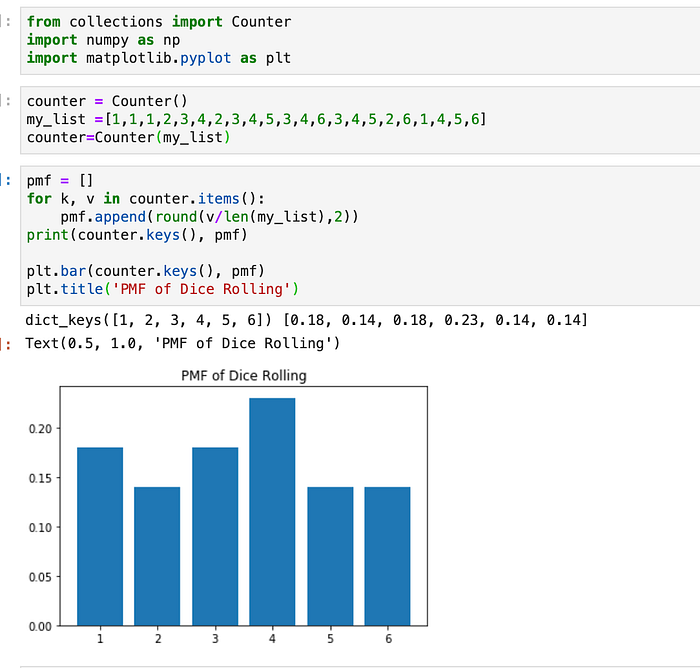
Lets make use the dice rolling as an example and calculate and plot the PMF in python:

When talking about distribution, there are two descriptive qualities to understand: expected value and variance. In discrete distributions:
Expected value: 𝐸(𝑋)=𝜇=∑𝑖𝑝(𝑥𝑖)𝑥𝑖
Variance: 𝐸((𝑋−𝜇)2)=𝜎2=∑𝑖𝑝(𝑥𝑖)(𝑥𝑖−𝜇)2
For the example above: E(X) = 1 * 0.18 + 2 * 0.14 + 3 * 0.18 + 4 * 0.23 + 5 * 0.14 + 6 * 0.14 = 3.46
Variance = 0.18*(1- 3.46)**2 + 0.14*(2–3.46)**2 + 0.18*(3–3.46)**2 + 0.23*(4–3.46)**2 + 0.14*(5–3.46)**2 + 0.14*(6–3.46)**2 = 2.4
Probability Density Function is applied when the probability distributions are continuous. PFD also called as probability distribution. FDS describes the possible values of an event, and the possibility of the values in theory is infinite.
Expected value: 𝐸(𝑋)=𝜇=∫+∞−∞𝑝(𝑥)𝑥𝑑𝑥E(X)=μ=∫−∞+∞p(x)xdx
Variance: 𝐸((𝑋−𝜇)2)=𝜎2=∫+∞−∞𝑝(𝑥)(𝑥−𝜇)2𝑑𝑥
Due to the possible values are infinite in PDF, the probability of a certain value does not exist. For example, in the distribution of temperature, The idea of continuous variables and PDFs is that the probability of any given arbitrary number is always 0, simply because there is an infinite number of possibilities .we can check (what is 𝑃(Temp=80.3)?P(Temp=80.3)? 𝑃(Temp=80)P(Temp=80.0002)?𝑃(Temp=80…5)?P(Temp=80.00000895)?) So, the probability of the temperature being exactly 80 Degrees is 0. When using a PDF, the only way of finding a probability associated with a certain temperature here is when using an interval of ranges, so something like:
𝑃(79.9<Temp<80.1)P(79.9<Temp<80.1)
Conclusion
Probability distribution is a foundational concept and practice in the statistics and machine learning. Understanding the most widely probability distribution and the PMF, PDF is very important in data science. I wish this brief introduction would help you. Thanks for reading.
